Quick Start Guide

PlateArrays.jl helps you place positive and negative controls on microwell plates. You provide the active wells on the plate and the number of controls to place; place_controls optimizes their locations and returns a PlateArray.

Create an active plate mask

A plate is represented by a BitMatrix mask, where true means a well is active (available) and false means it is inactive.

For a full 96-well plate:

wells = trues(8, 12)

For a full 384-well plate:

wells = trues(16, 24)

You can also mark some wells as inactive. For example, to exclude the first and last columns:

wells = trues(8, 12)

wells[:, 1] .= false
wells[:, end] .= false

Placing controls on a single plate

Use place_controls with the plate mask, the number of positive controls, and the number of negative controls.

plate = place_controls(wells, 8, 8)

This places 8 positive controls and 8 negative controls on the active wells of the plate.

The result is a PlateArray:

PlateArray objects

A PlateArray stores three BitMatrix objects:

plate.wells
plate.positives
plate.negatives

plate.wells indicates active wells.
plate.positives indicates positive control wells.
plate.negatives indicates negative control wells.

Visualizing PlateArrays

Use plot to visualize the plate. By default, positive controls are outlined in blue, and negative in red.

plot(plate)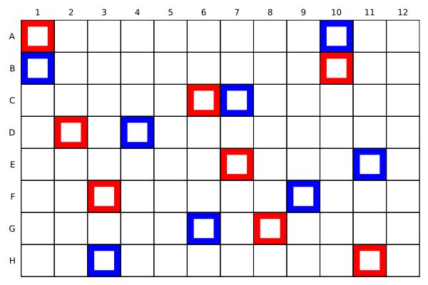

If a well is inactive, it will appear in a gray color.

Exporting PlateArrays

A PlateArray can be exported as a DataFrame

plate_df = DataFrame(plate)

well	row	col	run	positive	negative
A1	1	1	false	false	true
B1	2	1	false	true	false
C1	3	1	true	false	false
D1	4	1	true	false	false

Likewise, a properly formatted DataFrame can be converted back into a PlateArray

new_plate = PlateArray(plate_df)

Choosing a solver

By default, place_controls uses the "exchange" solver.

plate = place_controls(wells, 8, 8)

This is equivalent to:

plate = place_controls(wells, 8, 8; solver = "exchange")

Available solvers are:

Solver	Description
`"exchange"`	Default exchange-based optimization solver.
`"MILP"`	Mixed-integer linear programming solver.

To use the MILP solver:

plate = place_controls(wells, 8, 8; solver = "MILP")

Note

The MILP solver has unpredictable run times and works best for plate sizes up to 96 well plates.

Choosing an objective

By default, place_controls uses the "hybrid" objective.

plate = place_controls(wells, 8, 8)

This is equivalent to:

plate = place_controls(wells, 8, 8; objective = "hybrid")

Available objectives are:

Objective	Description
`"hybrid"`	Default weighted combination of the `minimax` and `LHS` objectives.
`"minimax"`	Minimizes the maximum distance from an active well to its nearest control.
`"LHS"`	Finds an approximate Latin hypercube sample of the available wells.

For example:

plate = place_controls(wells, 8, 8; objective = "minimax")

You can combine solver and objective choices:

plate = place_controls(
    wells,
    8,
    8;
    solver = "exchange",
    objective = "minimax",
)

Placing controls with `Experiment` objects

Experiment objects wrap the number of runs, positive controls, and negative controls into a single object.

experiment = Experiment(80, 8, 8)

This represents:

80 experimental runs
8 positive controls
8 negative controls

You can also call place_controls with Experiment objects.

wells = trues(8, 12)

experiment = Experiment(80, 8, 8)

plate = place_controls(wells, experiment)

Scheduling multiple experiments with `arrayer`

Use arrayer to schedule multiple experiments across one or more plates.

plate_arrays = arrayer(wells, experiment1, experiment2, experiment3)

arrayer executes three scheduling tasks:

Assigns experiments to as few plates as possible.
Partitions plates that contain multiple experiments.
Places the requested positive and negative controls for each experiment on each plate with place_controls.

The result is a matrix of PlateArray objects with dimensions E × P, where:

E is the number of experiments
P is the number of plates used

Each entry plate_arrays[e, p] contains the layout for experiment e on plate p.

Example: arraying multiple experiments

using PlateArrays

# Define a full 96-well plate.
wells = trues(8, 12)

# Define several experiments.
expt1 = Experiment(40, 4, 4)
expt2 = Experiment(32, 4, 4)
expt3 = Experiment(80, 8, 8)

# Assign experiments to plates and place controls.
plate_arrays = arrayer(wells, expt1, expt2, expt3)

Inspect the number of experiments and plates:

size(plate_arrays)

The first dimension corresponds to experiments, and the second dimension corresponds to plates.

For example:

plate_arrays[1, 1]

returns the PlateArray for the first experiment on the first plate.

If an experiment is not assigned to a particular plate, the corresponding PlateArray will contain no active wells.

Example: irregular plates

The active wells do not need to form a full plate. This example excludes the outer border of a 96-well plate:

using PlateArrays

wells = trues(8, 12)

wells[1, :] .= false
wells[end, :] .= false
wells[:, 1] .= false
wells[:, end] .= false

plate = place_controls(wells, 4, 4)

Controls are placed only where wells is true.